Learning without a label

Lecture 10 · room 202

Prof. Niccolò Salvini

HEMA · Università Cattolica del Sacro Cuore, Rome

Monday 2 November 2026

Today

Time		Min
17:00	Who I am, who you are	10’
17:10	Where we are · two dialects, statistics to AI	15’
17:25	The unsupervised problem	15’
17:40	RStudio: panes, running code, projects	20’
18:00	Break	10’
18:10	From a database to a dataset	25’
18:35	Setup check · Mac or Windows · already installed?	25’

Who I am

Statistics in the morning, for clients. Statistics in the evening, for you. Same subject, very different deadlines.

Who are you?

Hands up if you have ever…

Nobody? Perfect, we start from zero. Everybody? Better still: this semester you find out what that code was doing.

Objectives

See what Module 2 adds to Module 1, and why it comes second
Speak both dialects, the statistician’s and the machine learner’s — and see how they led to AI
State the unsupervised problem precisely — and see why it is harder to grade
Tell a database from a dataset, and read a dataset’s size, types and scale
Work inside an RStudio project, and know where R is looking for your files
Check that R, RStudio and the course packages run on your machine

Section 1 Where we are

Module 1 gave you a target

Every method so far had a y

Regression: a number to predict — sales, length of stay, cost
Logistic and Poisson: a class or a count
Time series: tomorrow, from yesterday
Ridge, LASSO: the same, with too many predictors

In every case the data came with the answer attached. The model’s job was to reproduce it.

Module 2 takes the target away — then gives it back

Weeks	Question	Has a y?
1–3	Which customers resemble each other? — clustering, PCA, correspondence analysis	No
4–6	Which will churn, default, be readmitted? — trees, forests, boosting, neural networks	Yes
7	Why did the model say that, and how do I tell the board?	—

The second half is supervised, like Module 1 — with algorithms in place of equations.

Section 2 Two dialects, one subject

The same things, with different names

Machine learning grew up next door to statistics and renamed the furniture

Statistics	Machine learning
Explanatory variable	Input, feature
Response variable	Output, target, label
Observations	Training set
Estimation, fitting	Training the model
Intercept	Bias
Transformation	Activation function
Coefficients, parameters	Weights

You will hear both in this room. They are the same objects.

Statistics, then machine learning, then AI

Three generations, asked the same four questions

Each column is built on the one before. This module: the first two.

Prediction is not inference — a manager’s version

Same model, two different questions

Inference: does a loyalty card increase spend, and by how much? — you need a coefficient you can trust, with an interval around it
Prediction: which of these 40 000 customers will spend most next quarter? — you need a ranking that holds up, and you do not care why

Module 1 was mostly the first question. Module 2 is mostly the second. Confusing them is the most common analytical mistake in business, and the most expensive.

Section 3 The unsupervised problem

No label, no error, no “correct”

The problem stated plainly

You have n rows and p columns — customers and their behaviour, patients and their measurements — and nothing to predict.

You are asked: is there structure? Do these rows fall into groups? Can p columns be summarised by fewer?

In supervised learning, a wrong prediction is a visible number: y - \hat y
In unsupervised learning there is no y. No residual, no accuracy, no test set.
Two analysts can produce two different segmentations of the same customers, and neither is wrong

Then how do you judge it?

Internal coherence: are the groups tight and far apart? (numbers exist — we will use them — but they measure geometry, not truth)
Stability: does the structure survive a different sample, a different seed, a different k?
Usefulness: can marketing act on the segments? Do clinicians recognise the patient groups?

Note

That last criterion is not a soft one. A segmentation nobody can act on is a wrong segmentation, however tight its clusters.

The three tools of the next three weeks

Tool	Question it answers	Business example
Clustering (k-means, hierarchical)	Which rows are alike?	Customer segments; patient case-mix groups
Principal components	Which few directions carry most of the variation?	The two or three drivers behind twenty survey items
Correspondence analysis	How do two categorical variables relate?	Brands × attributes — the perception map

All three are descriptive. They organise data; they do not predict anything. That is their strength and their limit.

Every unsupervised method is a choice you make.

What counts as “similar” is decided by you, not by the data.

Section 4 Finding your way around

R is the language. RStudio is the room you use it in.

RStudio is an IDE: it starts R and talks to it. You will always open RStudio, never R. Same split elsewhere: Python is the language, VS Code the room.

The four panes

You will spend the semester in 1 and read the results in 2. Panes 3 and 4 are for checking.

Where is R looking?

The working directory: the one folder R reads from and writes to, unless told otherwise

getwd() tells you where R is looking. Most “file not found” errors in this course are this slide.

A project is a folder R opens in

Double-click sbd_26_27.Rproj and RStudio opens there — or File ▸ Open Project. The setup script already made yours.

Three habits, from today

Do	Don’t
One project per course: `sbd_26_27`	Loose scripts on the Desktop
Data in `data/`, read with `here("data", "file.csv")`	`setwd("C:/Users/anna/Desktop/...")` — a path that exists on one computer on Earth
Open the project first, then the script	Open a `.R` file by double-clicking it: R starts in the wrong folder

The exam machines are not your laptop. A project plus here() is why your script will still run there.

Script or console?

Console	Script
type a line, Enter, see the answer	write lines in a file, run them when you choose
gone when you close RStudio	saved, rerunnable, shareable
for trying something	for keeping something

Habit to build this week: everything that matters goes in the script. The console is a scratchpad. Cmd/Ctrl + Enter runs the line your cursor is on; Cmd/Ctrl + Shift + Enter runs the whole script.

Running code: select, then Run

Notebook or script?

You will meet both.

A script (.R) is code, top to bottom. What we use in class, in labs, and in the exam.
A notebook (.qmd, .Rmd, Jupyter) mixes text and code cells with their output, in one document. Good for a report; the course site’s slides are one.
Same language inside. The notebook adds prose and layout around the code; it does not change what the code does.

Start with scripts. The notebook is a second thing to learn once the first is comfortable.

Reading an error without panic

> library(tidyvers)
Error in library(tidyvers) : there is no package called 'tidyvers'

Read the last line first. It names the problem: no package called tidyvers.
Find your typo, or your missing step. Here: a letter. Often: you loaded before installing, or the file is not where you think.
Copy the exact message into a search — or, this year, into an assistant. Then check the answer against what you know.

Attention

Red text in the console is R talking to you, not R breaking. A warning lets the code run and tells you something odd happened. An error stops it. Learn which one you got before you do anything.

Five words you will hear all semester

Word	What it is	You will see it as
object	anything with a name: a number, a table, a model	`fit`, `cust`, `X`
function	a verb: takes inputs, returns an output	`kmeans(X, 4)`
argument	an input to a function	`centers = 4`
package	someone else’s functions, installed once, loaded per session	`library(tidyverse)`
data frame	a table: rows are cases, columns are variables	`cust` from `read_csv()`

Everything on this slide you will use on Tuesday. Nothing else about programming is required before then.

Section 5 From a database to a dataset

Database ≠ dataset 😡

Three different objects. Mix them up and you will see this face again

	Database	Dataset	Data frame
What	linked tables, always changing	one table, one question, frozen	the dataset, inside R
Lives	on a server, behind SQL	in a file: `customers.csv`	in the Environment pane
Example	the bank’s core system	40 000 customers × 12 columns	`cust`

database → query → dataset → read_csv() → data frame

You never analyse a database. You analyse a dataset someone extracted from it — and which rows, dates and columns they took was already a choice.

How big is big data?

A dataset can grow in two directions, and each breaks something different

Big data usually lives in a database. What you analyse is still a dataset that fits on your laptop.

Columns have types

Type	Column	You can…
Numeric, continuous	`monthly_charge`, `tenure_months`	average, subtract, measure distance
Numeric, count	`support_calls`	the same, in whole numbers
Categorical, nominal	`region`, `payment`	count, tabulate; no mean
Categorical, ordinal	`contract`: month-to-month < … < two-year	rank; gaps not equal
Categorical, binary	`churn`: yes / no	the target, from week 4

The type decides what you may do. churn.csv: 7 numeric, 13 categorical columns — and clustering and PCA want numbers.

Five lines you need on Tuesday

library(tidyverse)                     # load the toolbox, once per session
cust <- read_csv("customers.csv")      # file → data frame; <- means "call it"
glimpse(cust)                          # every column, its type, first values
cust$monetary                          # one column: data frame $ column name
summary(cust$monetary)                 # a function applied to that column

   Min. 1st Qu.  Median    Mean 3rd Qu.    Max.
   41.0   267.0   568.0   796.6   991.2  9214.0

<- gives a name. $ picks a column. f(x) applies a verb. That is most of the grammar.

Scale decides who is “close”

Two real customers, and what their distance is made of:

Column	Customer A	Customer B	Share of the distance, raw	after `scale()`
`recency` (days)	35	251	8%	48%
`frequency` (orders)	14	3	0%	29%
`monetary` (€)	607	1 338	92%	5%
`tenure`, `returns`, `online`	…	…	0%	18%

Raw, the distance is spending. After scale() every column counts in standard deviations — and A and B differ because one bought last month, one eight months ago.

Train and test, on real customers

churn <- read_csv("churn.csv")          # 7 000 customers, 28.5% churned
set.seed(1)                             # same random split for everyone
idx   <- sample(nrow(churn), 0.7 * nrow(churn))
train <- churn[idx, ]                   # 4 900 rows: the model learns here
test  <- churn[-idx, ]                  # 2 100 rows: locked until the end

	Rows	Churn rate
`train`	4 900	28.7%
`test`	2 100	28.1%

Same customers, split at random: the two halves look alike. Any gap between the model’s score on train and on test is the model, not the data. Look at the test set once.

Section 6 Setup check

Ten minutes, now, on your own machine

Open RStudio, paste into the Console:

source("https://sbd-26-27.netlify.app/materials/setup.R")

library(tidyverse)
library(cluster)
library(factoextra)

fviz_nbclust(scale(USArrests), kmeans, method = "wss")

If a plot appears, you are ready for Tuesday. If not, that is what the next ten minutes and office hours are for — not Tuesday’s lab.

Before the lab

Bring a laptop that runs the line above. Nobody discovers a missing package in a lab; they discover it tonight.

Already installed? Check, don’t reinstall

R.version.string          # needs "R version 4.6" or newer

R older than 4.6? Install the new R from CRAN over it. Your scripts survive; your packages do not — the next line puts them back
RStudio: Help ▸ Check for Updates. It updates separately from R: updating one never updates the other
Then the same line as everyone else. It installs only what is missing and changes nothing that works — running it twice is harmless:

source("https://sbd-26-27.netlify.app/materials/setup.R")

Mac or Windows: what actually differs

	Mac	Windows
Shortcuts	`⌘`	`Ctrl`
Settings	`RStudio ▸ Settings`	`Tools ▸ Global Options`
Installer trap	arm64 (M1 on) vs Intel: pick right	needs admin rights
Paths	`/Users/anna/...`	`C:\Users\...`: backslashes break R — use `here()`
Quiet killer	iCloud Desktop sync	OneDrive: setup keeps you out of it

All the rest is identical. Details and screenshots: the Setup page — reread it at home, calmly.

Reading

ISLR chapter 12, §12.1–12.2 — unsupervised learning, PCA
Provost & Fawcett chapter 6 — similarity, neighbours, clusters: read this one for the business framing
Optional: ISLR chapter 2, §2.1.4 — supervised vs unsupervised, two pages

Appendix Make RStudio yours

Dark, rainbow, piped

Where the switches are

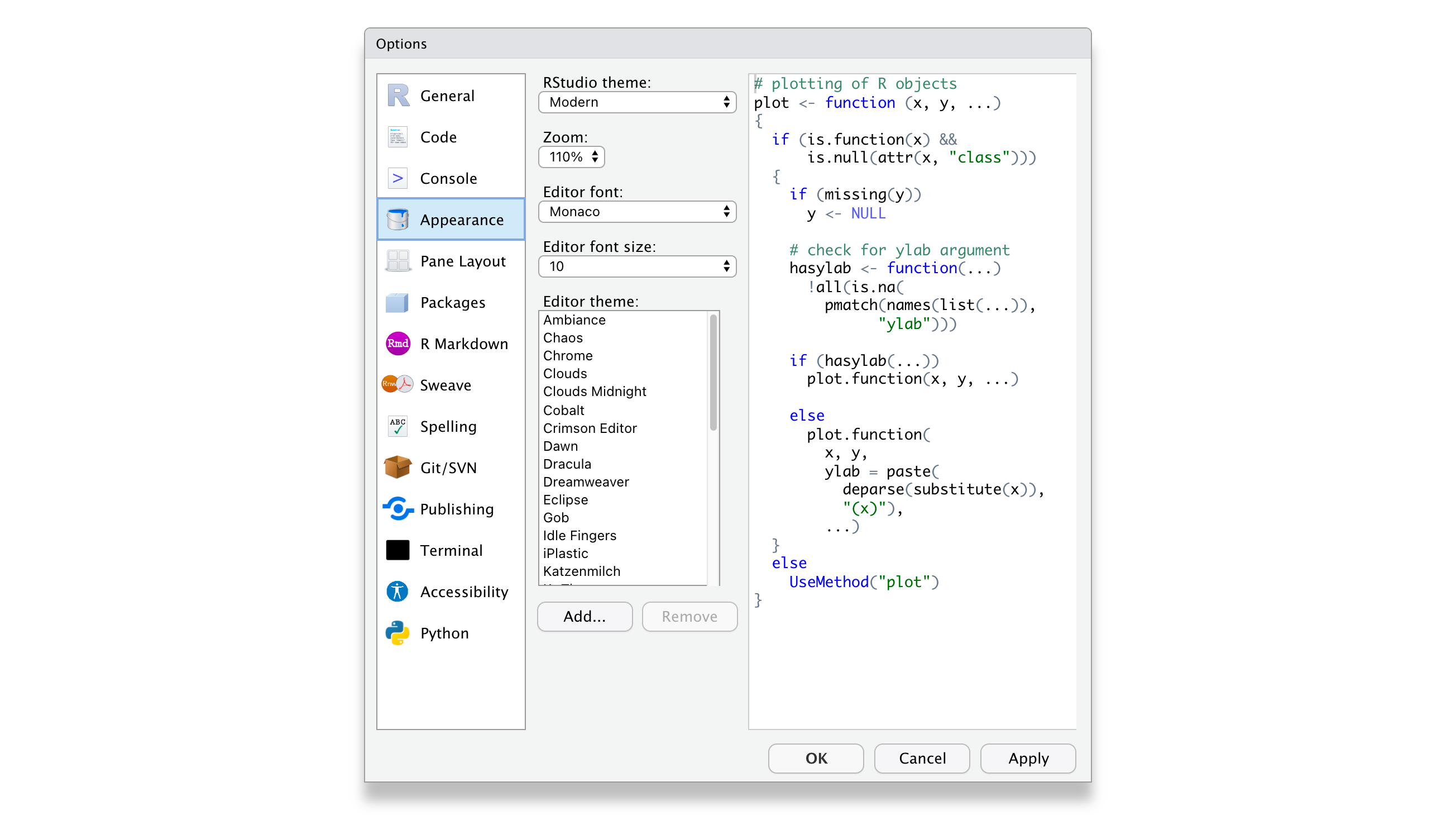
Tools ▸ Global Options · Mac: RStudio ▸ Settings

Appearance: theme, font, zoom. On the desktop app, install Fira Code or JetBrains Mono for ligatures: |> and <- become single glyphs
Code ▸ Display: rainbow parentheses, indent guides, highlight function calls
Code ▸ Editing: Use native pipe operator — then ⌘/Ctrl ⇧ M types |>
Pane Layout: console on the right, if you prefer a wide editor

Shortcuts that make you look fluent

Keys (Windows: `Ctrl` for `⌘`)	Does
`⌘ ⏎`	run the line, or the selection
`⌥ -` (Windows `Alt -`)	types `<-`
`⌘ ⇧ M`	types the pipe, `\\|>`
`⌘ ⇧ C`	comment / uncomment the selection
`⌘ ⇧ F10`	restart R — the honest test that your script runs from scratch
`⌘ ⇧ P`	the command palette: type what you want, RStudio finds it
`Tab`	complete a function, a column or a file name

Nobody is graded on their theme. But the restart shortcut will save you once before the exam.

More tricks: writing code

Keys (Windows: `Ctrl` for `⌘`, `Alt` for `⌥`)	Does
`⌥ ↑` / `⌥ ↓`	move the line up or down
`⌘ ⌥ ↑` / `⌘ ⌥ ↓`	copy the line above or below
`⌘ D`	delete the line
`⌥` + drag	rectangular selection: edit ten lines at once
`⌘ I` · `⌘ ⇧ A`	re-indent · reformat the selection
`⌘ ⌥ ⇧ M`	rename a variable everywhere it appears in the script
`Tab` inside `"…"`	completes a file name: no more typos in paths

More tricks: finding your way

Keys	Does
`# Load data ----`	four dashes make a section; `⌘ ⇧ O` shows the outline
`F1` on a function	its help page, without leaving the script
`F2` on a function	jumps to where it is defined
`Ctrl .`	go to any file or function in the project by name
`⌘ ↑` in the Console	your past commands, filtered as you type
`View(cust)`	the data frame as a spreadsheet
`⌥ ⇧ K`	every shortcut there is

Appendix R in one page

Vectors, tables, missing values

x <- c(607, 1338, 325, NA)       # a vector: c() combines values of one type
x[2]                             # 1338 — R counts from 1, not 0
mean(x)                          # NA: one missing value poisons the result
mean(x, na.rm = TRUE)            # 756.67 — say what to do with it
class(cust$monetary)             # "numeric"; class(churn$region) is "character"

cust[1:3, ]                      # rows 1–3, every column      table[rows, columns]
cust[, c("recency", "monetary")] # every row, two columns
cust[cust$monetary > 5000, ]     # the rows that pass a condition

Square brackets read as table [which rows, which columns]. An empty side means “all”.

The five verbs, and the pipe

cust |>
  filter(recency < 90) |>                         # keep rows
  select(id, frequency, monetary) |>              # keep columns
  mutate(avg_order = monetary / frequency) |>     # add a column
  group_by(frequency > 10) |>                     # split into groups
  summarise(n = n(), spend = mean(monetary))      # one row per group

Verb	Question it answers
`filter` · `select`	which rows · which columns
`mutate`	what new column do I need
`group_by` + `summarise`	what is the number, per group

Factors, and one plot template

churn$contract <- factor(churn$contract,
  levels = c("month-to-month", "one-year", "two-year"))   # categories, in your order
table(churn$contract)                                     # counts per category

ggplot(cust, aes(x = recency, y = monetary)) +   # data, and which column goes where
  geom_point(alpha = 0.3) +                      # what to draw
  labs(x = "Days since last purchase", y = "Spend (€)")

Every ggplot is the same three parts: data, aesthetics (aes: what goes on which axis), geometry (geom_: points, bars, lines). Change one, keep the others.

Appendix Module 1, in R

What Prof. Arbia did, and the line that does it

Question	Function	Read in the output
Mean equal to a value?	`t.test(x, mu = 750)`	`p-value`, 95% interval
Two groups differ?	`t.test(y ~ group)`	interval of the difference
Three or more groups?	`summary(aov(y ~ group))`	`F value`, `Pr(>F)`
y against one x	`lm(y ~ x)`	`Estimate`, its p-value
…holding others fixed	`lm(y ~ x1 + x2 + x3)`	`Adjusted R-squared`
Redundant predictors?	`car::vif(fit)`	above 5–10 is trouble
A yes/no target	`glm(y ~ ., family = binomial)`	`exp(coef(fit))`

Next slides: each one run on customers.csv or churn.csv.

One mean, two means

t.test(cust$monetary, mu = 750)                 # is average spend 750 €?

t = 4.4405, df = 5999, p-value = 0.000009137
95 percent confidence interval:  776.0  817.1

cust$online <- cust$channel_online > 0.5        # TRUE for mostly-online customers
t.test(monetary ~ online, data = cust)          # Welch: unequal variances, by default

t = 40.171, df = 5997.8, p-value < 2.2e-16
mean in group FALSE  mean in group TRUE
          1038.2842            351.5777

The interval does not contain 750, so we reject. Mostly-online customers spend about €690 less — the interval says between 653 and 720.

ANOVA: three groups or more

fit <- aov(monthly_charge ~ contract, data = churn)
summary(fit)

              Df  Sum Sq Mean Sq F value Pr(>F)
contract       2     237   118.5   0.177  0.838
Residuals   6997 4684482   669.5

tapply(churn$monthly_charge, churn$contract, mean)   # 65.5, 65.1, 65.4

p = 0.84: no evidence of a difference. Contract type does not change the monthly charge. An honest ANOVA often says no — and then TukeyHSD(fit) has nothing to find.

Simple, then multiple regression

lm(monetary ~ frequency, data = cust) |> summary()
lm(monetary ~ frequency + recency + tenure + returns, data = cust) |> summary()

	Simple	Multiple
`frequency` estimate	−41.3	−8.0
`recency`	—	+5.5 per day
`tenure`	—	+9.2 per month
`Adjusted R-squared`	0.072	0.447

The frequency effect shrinks by four fifths once recency enters: alone, it was carrying recency’s effect too. Adjusted R² penalises each extra predictor; here it barely moves from the plain R² (0.4472 → 0.4468) because 6 000 rows can afford four predictors.

Collinearity: are two predictors saying the same thing?

round(cor(cust[, c("frequency", "recency", "tenure", "returns")]), 2)
car::vif(fit)          # install.packages("car") once

frequency   recency    tenure   returns
 1.785508  1.494547  1.206512  1.160302

VIF = 1 / (1 − R²) of each predictor regressed on the others. 1 is no overlap; above 5–10 the standard errors inflate and the coefficients start swapping signs from sample to sample. Here, all below 2: the four predictors carry distinct information.

Logistic regression: a yes/no target

churn$churn <- factor(churn$churn)                 # models "yes"
fit <- glm(churn ~ tenure_months + contract + monthly_charge,
           data = churn, family = binomial)
exp(coef(fit))                                          # odds ratios
predict(fit, newdata = tibble(tenure_months = 3, contract = "month-to-month",
                              monthly_charge = 90), type = "response")

  tenure_months contractone-year contracttwo-year  monthly_charge
          0.990            0.313            0.121           1.011
                                                          → 0.535

A two-year contract cuts the odds of leaving by 88% (0.121). A new, month-to-month, €90 customer: 53.5% chance of churning. That last number is where Module 2 picks up — with trees and forests instead of one equation.